DonorsChoose — funding risk and deep feature synthesis

The first three tutorials had a secret advantage: strong signal. Chicago 311’s sr_type practically is the answer (AUC ≈ 0.9). DonorsChoose (KDD Cup 2014) is the honest opposite — diffuse signal spread across many weak features, top AUCs in the 0.70s — which makes it the right dataset for the questions this page teaches: how do you build features from a multi-stream entity graph, and how do you find out which feature family actually carries the lift?

Prerequisites: the smoke test; the framing vocabulary from DirtyDuck.

The case

Teachers post classroom projects — books, microscopes, field trips — with a price tag; donors fund them. Some projects reach their goal in days; about a third never get fully funded. Knowing at posting time which projects will struggle lets the platform intervene early: featuring, matching offers, coaching on the ask.

The question: will this newly-posted project still be unfunded four months from now? (The positive class is the project that needs help.)

task_framing: early_warning   # funding outcomes are recorded for every project

The data — and the leakage trap it sets

just donors-up          # ~3,000 real projects (2012–13) baked in; full Kaggle data mountable
uv run triage --dbfile donorschoose-database.yaml db upgrade

The ontology layer is a four-entity graph around projects:

• ontology.entities = projects — the target; static attributes (grade level, subject, poverty level, price) known at posting;
• resources — the line items of the ask (books? technology? how many, at what price) — known at posting, a legitimate child stream;
• teacher history / school history — prior projects by the same teacher or school, reached self-referentially through teacher_acctid / schoolid;
• donations — the label source only. Never a feature. At posting time a project has zero donations by definition; any donation-derived feature is pure leakage dressed as signal. The config never references the donations table in feature_config, and that absence is a design assertion, not an oversight.

The label compares four months of donations against total_price:

(coalesce(sum(donations within {label_timespan}), 0) < total_price)::int

Features — a real entity graph, all as-of

This is the deepest feature_config in the tutorials — one target with three child streams, each joined as-of so only what existed before the as_of_date counts:

• projects.* — one-hot categoricals + numerics of the ask itself;
• resources.* — aggregations over the line items (counts, price stats, type mix);
• teacher_history.* — the same teacher’s prior projects: how many, how often funded, typical price. A first-time teacher has no rows — which is itself information, handled by the imputation rule, not by peeking;
• school_history.* — the same, at the school grain.

featurizer expands this to ~30 features across the four families. The histories are the subtle ones: “teacher’s past funding rate” is computed as of each posting date from projects posted strictly before — a self-referential as-of join you’d have to hand-write very carefully in raw SQL, and get silently wrong the first time.

Run it — then ask which family matters

uv run triage --dbfile donorschoose-database.yaml run \
  example/donorschoose/experiment.yaml --project-path /tmp/donors-run

(6 model groups × 4 splits = 24 models on the baked subset — the five real estimators plus the constant-prior DummyClassifier floor; base rate ≈ 0.32.)

Now the chapter this dataset exists for. Uncomment the feature_groups block in the config (it ships commented, inside feature_config):

feature_config:
  # …the entity graph…
  feature_groups:
    group_by: source_entity
    strategies: [all, leave-one-out]

and re-run. One experiment fans out into five runs — the problem hash does not change (features are the attempt, not the problem), so their leaderboards are directly comparable:

  run 0cb379da… (all):                            24 model(s)
  run 3f32af45… (leave-one-out:projects):         24 model(s)
  run 49c1d0ce… (leave-one-out:resources):        24 model(s)
  run bf24745c… (leave-one-out:school_history):   24 model(s)
  run d644f9d9… (leave-one-out:teacher_history):  24 model(s)

Each leave-one-out:X run trains without family X. Read the comparison in the dashboard’s Model Groups tab (or triage models <hash>): if dropping teacher_history barely moves the metric, its lift is redundant with the others; if dropping projects craters it, the ask’s own attributes carry the model. On the baked subset the differences are small and noisy — top AUCs sit in the low-to-mid 0.70s whichever family you drop — and that is the finding: diffuse-signal problems are exactly where feature-family ablations save you from over-narrating any single feature’s importance. (With the full 1.6 GB Kaggle data mounted, the contrasts sharpen.)

The cohort, labels, and shared feature artifacts cache-hit across all five runs — the fan-out costs marginal training time, not a pipeline rebuild.

Reading a diffuse-signal leaderboard

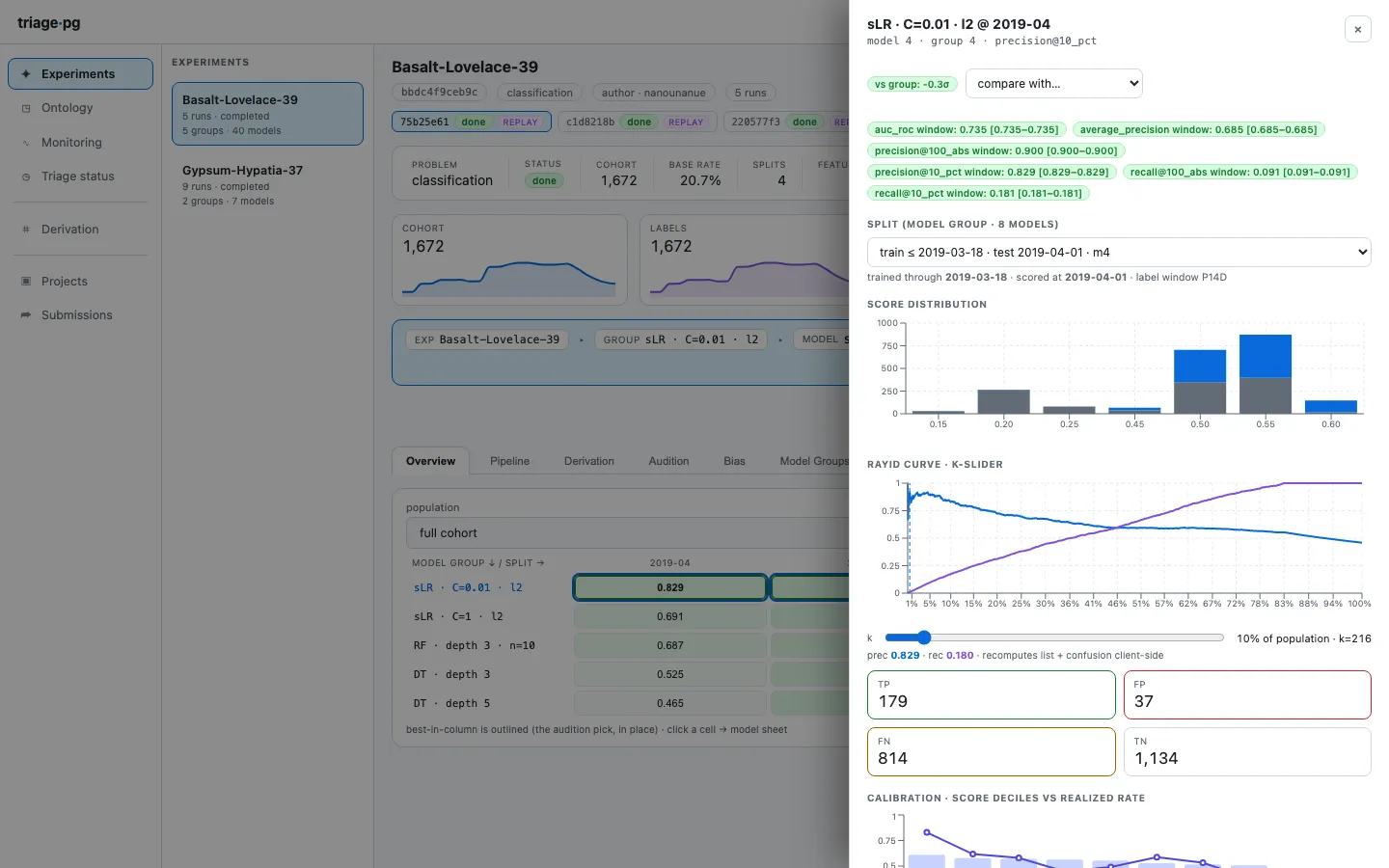
Two habits this dataset rewards:

• Look at stability, not the single best cell. With weak signal, the per-split winner shuffles; audition’s regret rules (triage audition) pick the group that is never far from best, which is the deployable property.
• Mind the base rate (≈ 0.32). Precision@k must beat it to mean anything; an AUC of 0.72 here is honest work, not a weak result — compare DirtyDuck’s inspections case (0.277 base, moderate lift) and 311’s structural signal (0.87+). Three datasets, three signal regimes: that calibration of expectations is the real deliverable of this series.
• Make the base rate a competitor, not a footnote. The committed grid ships the constant-prior DummyClassifier on the leaderboard next to your models — the floor a real model must clear:

grid_config:
  # ... your real estimators ...
  'sklearn.dummy.DummyClassifier':
    strategy: ['prior']

On a diffuse-signal problem this is the most important row in the grid (per-algorithm averages across the 4 splits):

model	AUC	AP	precision@100
RandomForestClassifier	0.597	0.413	0.330
DecisionTreeClassifier	0.596	0.424	0.332
ScaledLogisticRegression	0.575	0.421	0.331
DummyClassifier (constant floor)	0.500	0.379	0.327

The real models clear the floor only narrowly — AP 0.42 vs 0.38, and every precision@100 sits right at the ≈ 0.33 base rate. Honest work on a hard problem, not a triumph.

The DSSG-original BaselineRankMultiFeature is worth a look too. Rank projects by the size of their ask (COUNT(resources.date)) and the plausible story — “bigger asks are harder to fully fund” — turns out anti-predictive on this subset: AUC 0.442, below the coin-flip floor. A rule can be worse than nothing, and you only find out by scoring it. (It ranks on a resources column, so don’t pair it with a feature_groups leave-one-out that drops that group — its feature must be in the matrix.) The full catalog (every problem_type, the time-series and survival floors) is the Baselines reference.

Where this differs from DSSG triage

DSSG’s DonorsChoose appearances (KDD-era baselines) hand-built aggregate features; here the four-family graph is nine lines of YAML per family and the ablation study is two. Feature-group strategies existed in DSSG triage too — triage-pg keeps the idea but makes each subset a first-class run of the same experiment, so provenance, caching, and the leaderboard treat the ablation as data, not as five separate experiments to bookkeep. The side-by-side has the rest.

Where next

You’ve now seen all three signal regimes and both observation regimes. From here:

• docs/quickstart.md §“your own data” — pointing triage-pg at your own PostgreSQL;
• the onboarding one-pager as the map of everything else;
• just donors-down when done.