How a feature is computed

featurizer reads a config, plans a set of features, renders one SQL query, and runs it. This page follows one small config through all four steps and shows the SQL each step emits, as 1.3.0 renders it. The walkthrough shows how to run it; the configuration reference lists every key; the ADR index records why each decision was taken. This page is about what happens in between.

The config used throughout:

target: customers
max_depth: 2
intervals: [P30D]
aggregations: [count, sum]
transformations: [identity, lag_1]

entities:
  - alias: customers
    id: customer_id
    table: customers
    temporal_ix: signed_up
    variables:
      age: {type: numeric}
  - alias: orders
    id: order_id
    table: orders
    temporal_ix: ordered_at
    variables:
      amount: {type: numeric}

relationships:
  - parent: {entity: customers, key: customer_id}
    child:  {entity: orders,    key: customer_id}

Every SQL fragment below is taken from Featurizer("config.yaml").query for this config, with whitespace trimmed; I paraphrased nothing.

1. The plan: a traversal of the entity graph

The planner starts at the target and walks the relationships up to max_depth. Along each relationship, features flow in one of two directions:

• Aggregation, child to parent. Many orders rows roll up onto one customers row through the selected aggregations. This is the direction of every relationship whose parent is nearer the target.
• Transfer, parent to child. A relationship marked temporal: {mode: as_of} (or a plain forward relationship) carries a parent’s columns onto each child row. The lookup table is the parent, the receiving entity the child.

At each entity the planner also runs the transformations, and, where the config declares them, the planner passes (peer groups, spatial and graph relationships), which read base tables in CTEs of their own. For the config above the plan is short: read orders, transform it, aggregate it onto customers, transform customers. The result is 18 output columns, listed in feature_manifest:

COUNT(orders.order_id)                     COUNT(orders.order_id|interval=P30D)
COUNT(orders.ordered_at)                   COUNT(orders.ordered_at|interval=P30D)
SUM(orders.amount)                         SUM(orders.amount|interval=P30D)
SUM(orders.LAG_1(orders.amount))           SUM(orders.LAG_1(orders.amount)|interval=P30D)
LAG_1(customers.COUNT(orders.order_id))    …one LAG_1 per column above, and LAG_1(customers.age)
age

Two things are visible already. Every aggregation yields a whole-history column and one column per interval (the |interval=P30D suffix; see the column budget). And transformations apply at every level: lag_1 runs on orders.amount before the aggregation, and again on every column of customers after it, which is where LAG_1(customers.COUNT(orders.order_id)) comes from.

2. The spine: one evaluation per as-of date

Everything hangs off the table you provide, as_of_dates:

select aod.as_of_date, t.*
from as_of_dates as aod
cross join lateral (
  with
    orders_synth as (…),
    orders_transform as (…),
    orders_aggs_for_customers as (…),
    customers_synth as (…),
    customers_transform as (…)
  select * from customers_transform
) as t
order by aod.as_of_date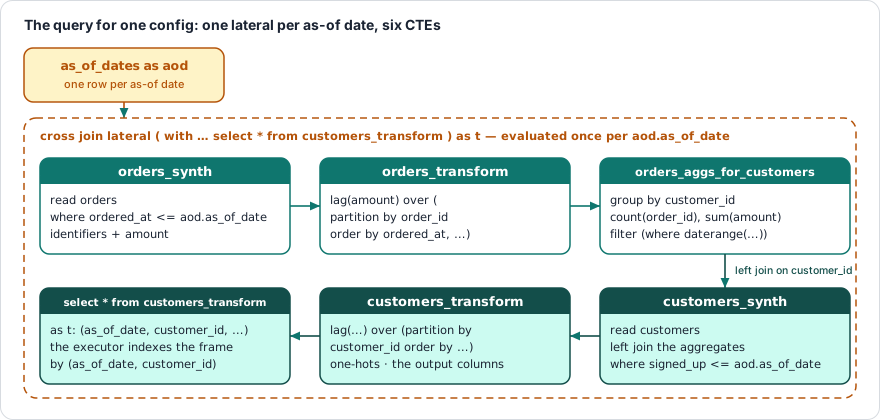

cross join lateral evaluates the whole with block once per as-of date, with aod.as_of_date in scope inside every CTE. That scope is what makes the rest of this page possible: any CTE can compare a row’s timestamp with the date the lateral is computing.

By default the query emits every target row under every date. When each date has its own set of entities, as_of_dates: {id_column: …} changes that; see paired cohorts and section 7.

3. Reading an entity: the cut on the as-of date

The first CTE of each entity reads its base table. That read is where the point-in-time guarantee lives:

orders_synth as (
  select
    orders."order_id", orders."ordered_at", orders."customer_id", "amount"
  from orders
  where orders."ordered_at" <= aod.as_of_date
)

Every entity that declares a temporal_ix is cut at the moment it is read, with <= aod.as_of_date (or < under as_of_boundary: exclusive). Nothing downstream of orders_synth can see an order dated after the as-of date, whatever it computes over the rows: a window over its whole partition, a population statistic, a run length.

That last sentence is the reason the cut sits here and not only in the aggregation. Until 1.3.0 the child was read whole and cut when aggregated; a backward-looking window never noticed, but percent_rank() divides by the size of its partition, and that size counted rows the aggregation was about to drop. Six transformers changed value for it; the 1.3.0 entry of the changelog lists them.

The target is read the same way. customers declares signed_up, so:

customers_synth as (
  select
    customers."customer_id", customers."signed_up", "COUNT(orders.order_id)", …, "age"
  from customers
  left join orders_aggs_for_customers
    on orders_aggs_for_customers."customer_id" = customers."customer_id"
  where customers."signed_up" <= aod.as_of_date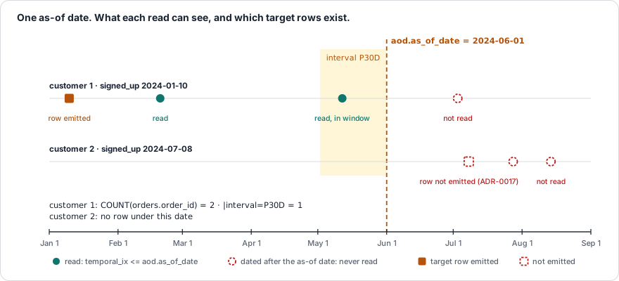
)

A customer who signs up in August is not a row under an as-of date in January. Their aggregates would have been NULL anyway; emitting the row told a model trained as of January that the customer would exist (since 1.3.0). A target without a temporal_ix is read whole, which is how you ask for every target row under every date. The planner logs one warning per process for a target that declares one, so the smaller row count is never a surprise.

4. Transform: windows, and the order they walk

The second CTE applies the selected transformations to the synth’s columns:

orders_transform as (
  select
    "order_id", "ordered_at", "customer_id",
    lag("amount", 1) over (partition by "order_id"
                           order by "ordered_at", "customer_id", "amount")
      as "LAG_1(orders.amount)",
    "amount" as "amount"
  from orders_synth _ego
)

Three things decide what a window computes.

The partition is the entity’s id. A window walks the rows that share one id. Here orders declares id: order_id, one row per order, so every partition has one row and LAG_1(orders.amount) is NULL on every row. To walk a customer’s orders in order, declare the child with the id of the thing whose history you want (id: customer_id). An entity with no id has no partition, and the window transformers emit nothing for it.

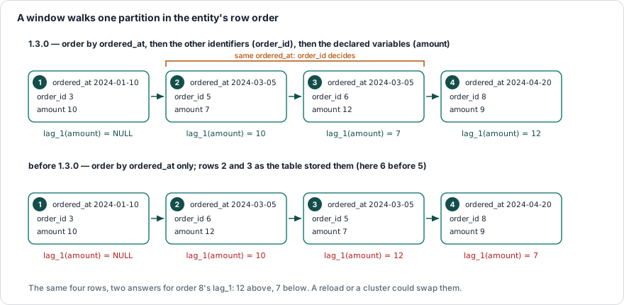
The order is the entity’s row order (since 1.3.0): the temporal index, then the entity’s other identifier columns (relationship keys and index-typed variables; the id is the partition), then every declared variable. For orders that is "ordered_at", "customer_id", "amount". Two rows on one timestamp are ordered by their identifiers and then by their values, so lag_1 returns the same value however the table happens to be stored. Before 1.3.0 the order was the temporal index alone, and two rows on one date came out in the physical order of the table; a reload or a cluster could change a lag, a transition or a run length. Every window of an entity uses the same list, so PostgreSQL sorts the entity once for all of them.

Rolling percentiles are a subquery, because PostgreSQL does not allow over on an ordered-set aggregate. rolling_median_7 re-reads the entity’s synth for the seven most recent rows up to and including the current one, in the same row order, and takes percentile_cont(0.5) over them.

Transformers other than windows are plain expressions over the row: abs("amount"), case when "amount" > 0 then ln("amount") end, the date parts. A transform never joins.

5. Aggregate: a group by on the join key

The third CTE reads the child’s transform, cut again on the date (the read is already cut, so this second where costs nothing), and groups by the child side of the relationship:

orders_aggs_for_customers as (
  select
    orders_transform."customer_id",
    count("order_id") as "COUNT(orders.order_id)",
    count("order_id") filter (where daterange((aod.as_of_date - interval 'P30D')::date,
                                              aod.as_of_date::date, '[]') @> "ordered_at"::date)
      as "COUNT(orders.order_id|interval=P30D)",
    sum("amount") as "SUM(orders.amount)",
    sum("amount") filter (where daterange(…) @> "ordered_at"::date)
      as "SUM(orders.amount|interval=P30D)",
    sum("LAG_1(orders.amount)") as "SUM(orders.LAG_1(orders.amount))",
    …
  from orders_transform
  where "ordered_at" <= aod.as_of_date
  group by "customer_id"
)

An interval is a filter (where …) on the aggregate, over a daterange that ends at the as-of date and is closed or half-open according to as_of_boundary. That is why an aggregation yields intervals + 1 columns: one aggregate call per interval plus the unfiltered one.

Not every aggregation fits a group by. A transition matrix, an autocorrelation, a run length or a spatial path needs the rows in order first. Those families render a companion pre-pass CTE (one per family and interval) that orders the child’s rows by the same row order as section 4, computes the per-row quantity (lag, a transition pair, a run id), and reduces it per key. The aggregation CTE then reads the companion’s result. Families that fall outside both shapes render a correlated subquery per target row, over the same order.

As-of lookups go the other way. When a relationship carries temporal: {mode: as_of}, the child’s synth gains a left join lateral that takes, for each child row, the parent row dated at or before the child’s own timestamp, within grace if one is set. Rendered for an events entity that looks up a rates table by zone, with grace: P90D:

events_synth as (
  select
    events."event_id", events."ts", events."series_id", events."zone", "rate", "x"
  from events
  left join lateral (
    select rates_transform."rate" as "rate"
    from rates_transform
    where rates_transform."zone" = events."zone"
      and rates_transform."valid_from" <= events."ts"
      and rates_transform."valid_from" >= events."ts" - interval 'P90D'
    order by rates_transform."valid_from" desc, rates_transform."rate_id" desc,
             rates_transform."rate" desc
    limit 1
  ) as rates_asof_for_events on true
  where events."ts" <= aod.as_of_date
)

The order by … desc runs over the source’s row order too, so two source rows on one timestamp always yield the same one (1.3.0). The transferred column is then a column of the child like any other, and its parent may aggregate it under intervals and count alike.

6. The target’s read, and the output

customers_synth (section 3) joins the aggregation CTE onto the target’s base table with a left join, so a customer with no orders keeps their row and gets NULL aggregates. NULL is kept as a signal, never filled in at this stage; the imputation contract is a separate, opt-in pass.

customers_transform is the output. It applies the transformations once more, over the target’s own variables and over every aggregate, and projects exactly the columns the manifest lists, in the manifest’s order. A target variable with role: categorical becomes its one-hot columns here, against a fixed vocabulary; the planner dropped one with role: identifier before synth. The final select * from customers_transform is what the lateral returns, and the executor indexes the frame by (as_of_date, customer_id).

Column names are the manifest’s column: the readable SUM(orders.amount|interval=P30D), or a hash-capped form when the readable name would pass PostgreSQL’s 63-byte limit. feature_manifest carries the full label and the lineage for every column, so select by label, never by parsing the column.

7. A paired cohort

With as_of_dates: {id_column: cohort_id} the table you provide holds (as_of_date, customer_id) pairs, and two reads change. aod ranges over the distinct dates, and the target’s read keeps the ids paired with the current date:

from customers
left join orders_aggs_for_customers on …
where customers."customer_id" in (select _cohort."cohort_id" from as_of_dates _cohort
                                  where _cohort.as_of_date = aod.as_of_date)
  and customers."signed_up" <= aod.as_of_date

A child that only the target aggregates is read for that cohort as well, as whole window partitions, so a date no longer aggregates the history of every customer to keep a twentieth of it. The paired cohorts page has the predicate for each graph shape, which children keep their full read, and the measurements. Without the block, nothing on this page changes.

8. Three render paths, one result

The query above is the single query, and it is what Featurizer.query returns while the output fits PostgreSQL’s limits. Two limits bind: a target list may hold 1,664 entries, and a heap row 8 kB. A config that passes either renders differently, with the same result:

• Column groups. The output is split into groups of columns; each group is a query of the shape above, pruned to the CTEs and joins its columns need, and every group leads with the target’s identifier columns. The executor re-joins the groups on those columns. query_groups returns them; query raises, because there is no single query to return.
• TEMP tables. When a child’s synth or transform is itself too wide, the executor materializes the chain into session TEMP tables before the group queries run, one shard per as-of date and column slice, in the single query’s own shape, and the group queries read the shards. materialization_ddl holds the statements.

The three paths agree on every value. That is a tested claim, not a design intent: tests/integration/test_path_equivalence_defaults.py runs the curated defaults through all three and compares the matrices, and the sharding tests compare each path against a narrow single query over the same tables.

9. What the executor does before the query runs

to_dataframe, to_arrow, to_parquet and to_tables share one preamble on the connection they run on:

1. analyze as_of_dates, savepoint-isolated, because a table you created seconds ago has no statistics and PostgreSQL would plan the lateral for a 2,550-row default.
2. set local jit = off, then the query, then your previous value back (1.3.0). PostgreSQL compiles every expression of a query over jit_above_cost before it reads a row, and a generated query is a target list of hundreds of aggregate expressions; on the three live validation databases the JIT was faster in no cell and up to 7.9× slower (internals). This is the one setting a connection you pass in sees changed.
3. Planner tuning (work_mem, the join collapse limits), on connections featurizer opens itself only, because set local would stay in force inside your transaction.

If you execute query or query_groups yourself, the first two are yours to do; the FAQ has the two statements.

10. The checks every primitive passes

Every registered aggregation and transformer runs against PostgreSQL under seven invariants, and a new primitive cannot land without its row (tests/test_sweep_matrix_coverage.py fails the fast tier otherwise):

invariant	what the sweep does
it executes	every primitive, on every input type it declares
a declared name is quoted wherever SQL reads it	a column called MEAN(games.goals), a temporal index called Event Date, in every role a name can have
a row dated after the as-of date moves nothing	the same query with and without a later row
the three render paths agree	the curated defaults through all three
a config that validates runs	fifteen generated shapes
a paired cohort equals the dense matrix on its pairs	every primitive, three id shapes, twelve graph shapes
a value does not depend on the physical order of the rows	the same rows inserted forwards and backwards, six series with three ties each

The table is the one in CONTRIBUTING.md, “The sweep matrix”, where each row names its test files.